
Internal Revenue Code Section 871(m) and the regulations thereunder treat “dividend equivalent payments” on certain equity derivatives as dividends from sources within the United States.[1] [2] That is, federal withholding tax applies to such payments made to non-U.S. parties.[3]
More specifically, the 871(m) regulations generally impose U.S. withholding tax on equity derivatives that reference one or more U.S. equities and that (i) have a delta greater than or equal to 0.8 (if the derivative is a “simple contract,” as explained below) or (ii) fail a “substantial equivalence test” (if the derivative is a “complex contract,” as explained below).[4]
A simple contract is, essentially, an equity derivative that has (i) a single, fixed number of shares of the underlying asset and (ii) a single exercise or maturity date.[5] A complex contract is, essentially, an equity derivative that is not a simple contract and, therefore, for which computing delta would be conceptually problematic, thus requiring application of the substantial equivalent test (“SET”).
Regarding the SET, the preamble to 2017 Release provides the following very high-level description:
Generally, the substantial equivalence test measures the change in value of a complex contract when the price of the underlying security referenced by that contract is hypothetically increased by one standard deviation or decreased by one standard deviation (each, a ‘‘testing price’’) and compares that change to the change in value of the shares of the underlying security that would be held to hedge the complex contract when the contract is issued (the ‘‘initial hedge’’) at each testing price. The smaller the proportionate difference between the change in value of the complex contract and the change in value of its initial hedge at multiple testing prices, the more equivalence there is between the contract and the referenced underlying security. When this difference is equal to or less than the difference for a simple contract benchmark with a delta of 0.80 and its initial hedge, the complex contract is treated as substantially equivalent to the underlying security. When the steps of the substantial equivalence test cannot be applied to a particular complex contract, a taxpayer must use the principles of the substantial equivalence test to reasonably determine whether the complex contract is a section 871(m) transaction with respect to each underlying security.[6]
The SET is described in greater detail below. The SET is considerably more elaborate than the 0.8 delta test and involves a degree of mathematical and statistical complexity uncharacteristic of the tax laws. This article attempts to provide a brief, but comprehensible overview of the SET.
- Simple Contracts and Measuring Delta
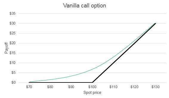
Before turning to the SET, a brief discussion of measuring delta for simple contracts is in order. As an example of a simple contract, the graph below depicts a vanilla call option. The black line represents payoff at maturity and the green line represents the fair market value of the call option at issuance. As reflected in the graph, the green line becomes increasingly steep as the spot price increases. At very low spot prices, the slope of the green line is nearly 0; at such levels, a small increase in the spot price of, for example, $1 results in a change in the payoff of little more than $0. Accordingly, the delta in such a case is approximately $0 / $1 = 0. By contrast, at very high spot prices, the slope of the green line is nearly 1; an increase in the spot price of $1 results in an increase in the payoff of a little less than $1. Accordingly, the delta in such a case is approximately $1 / $1 = 1. Between those two extremes, at a spot price of $100 (the “at-the-money” spot price), the delta is approximately $0.50 / $1 = 0.5.
- Complex Contracts and Applying the SET
The applicable regulations generally define “complex contract” as any derivative that references one or more U.S. equities but that is not a simple contract.[7] Depending on the type of complex contract, various conceptual problems may preclude application of the 0.8 delta test. For example, holding a structured note that provides a 200% possible upside return and a 100% possible downside return is economically equivalent to being long two call options and short one put option. In calculating the delta for such a structured note, it is unclear whether the denominator component of the delta ratio should equal a small change in one share of the underlying asset or a small change in two shares of the underlying asset. The component of the structured note consisting of two long call options implies that two is the appropriate number, whereas the component consisting of one short put option implies that one is the appropriate number. Other types of complex contracts, including digital options or structured notes with knock-in or knock-out features, present similar problems for measuring delta.
To understand the rationale for the SET, assume that a non-U.S. investor wishes to purchase and receive dividends on a U.S. equity security. To do so, the investor could directly purchase the desired amount of the U.S. equity security (“strategy A”). Alternatively, the investor could enter into a derivative that was economically comparable to strategy A (“strategy B”).
For small changes in the price of the U.S. equity security, the payoff of strategy A would be essentially the same as the payoff of strategy B. However, for larger changes in price of the U.S. equity security, the two payoffs could differ substantially, in which case the investor would be more likely to conclude that strategy B is not an acceptable alternative to strategy A.
As illustrated in the graph below, the SET examines the difference between strategy A and strategy B given probable changes in the price of the underlying asset. The graph depicts a structured note that is equivalent to being long an “up-and-out” call option (i.e., a call option ceases to exist if the price of the underlying asset increases beyond a specified price) and short a “down-and-in” put option (i.e., a put option that exists only if the price of the underlying asset decreases beyond a specified price). The solid black line represents the payoff of the complex contract at maturity. The green line represents the payoff of the complex contract at issuance. The dashed line represents the payoff of the initial hedge of the complex contract.[8] Because of its hedging function, the initial hedge should resemble Strategy A and involve the same number of shares that would be purchased in Strategy A.
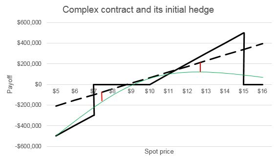
The difference between the value of the complex contract at issuance and the value of the initial hedge is represented by the two red lines. The red lines are placed one standard deviation below and one standard deviation above the spot price of the underlying equity security at issuance of the complex contract.[9] Because the dashed lined indicates the values of strategy A and the green line indicates the values of strategy B, shorter red lines imply greater equivalence between the two strategies.
The lengths of the red lines are then multiplied by the probabilities that the price will increase or decrease, as applicable, from the spot price at issuance. Those numbers are then added together and divided by the number of shares of the underlying asset used in the initial hedge. These adjustments produce a single number that will be appropriately scaled to be compared against the corresponding number for the benchmark instrument, as described below.
The SET then similarly examines a “benchmark instrument,” defined as:
. . . an actual or hypothetical simple contract that, at the calculation time for the complex contract, has a delta of 0.8, references the applicable underlying security referenced by the complex contract, and has terms that are consistent with all the material terms of the complex contract, including the maturity date. If an actual simple contract does not exist, the taxpayer must create a hypothetical simple contract. Depending on the complex contract, the simple contract benchmark might be, for example, a call option, a put option, or a collar.[10]
Given the terms of the complex contract in this case, a call option is the appropriate benchmark instrument. In the graph below, the solid black line represents the payoff of the call option at maturity, the green line represents the payoff of the call option at issuance, and the dashed line represents the payoff of the initial hedge of the call option.
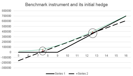
The SET compares the payoff of the call option at issuance to the payoff of the initial hedge, in the same manner as for the complex contract and its initial hedge, as described above. Again, the lengths of the red arrows are multiplied by the relevant probabilities, and then added together, and then divided by the number of shares of the underlying asset used in the initial hedge.
Because the benchmark instrument has a delta of 0.8, this final number for the benchmark instrument can be understood as a threshold that is derived from the 0.8 delta test for simple contracts. Accordingly, if the final number for the complex contract exceeds the final number for the benchmark instrument, the complex contract “passes” the SET and is not treated as an 871(m) transaction.
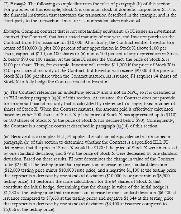
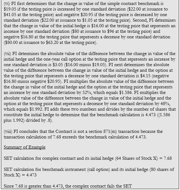
The regulations under 871(m) provide a detailed numerical example the SET, which is provided in the box below in full.[11] The example presents a SET analysis for a complex contract that fails the SET. In the example, the absolute values of the differences between the change in value of the initial hedge and the complex contract at the two testing prices (i.e., one standard deviation up and one standard deviation down) are $720 and $244. In the graphical approach taken above, these amounts would be represented by the red arrows in the graph relating to the complex contract and its initial hedge. After multiplying those amounts by the relevant probabilities, and then summing the amounts together and dividing by the number of shares that constitute the initial hedge, the ultimate calculation is 7.68. The equivalent calculation for the benchmark instrument is 4.473. Because 7.68 exceeds 4.473, the complex contract fails the SET and will not be subject to the 871(m) withholding requirements. The numerical example can be read in light of the conceptual background provided in this article.

[1] The graphical approach taken in this article is based on a presentation by Richard Maile at the International Fiscal Association USA New York Region Fall Seminar on December 7, 2015. Section 871(m) regulations have been discussed in previous Derivatives in Review postings (available here, here, and here).
[2] The Section 871(m) regulations apply to delta-one transactions issued on or after January 1, 2017 and will apply to non-delta-one transactions issued on or after January 1, 2018. See Dividend Equivalents from Sources Within the United States, 82 Fed. Reg. 8,144, 8,154-55 (January 24, 2017) (the “2017 Release”).
[3] For some time, parties to ISDA Master Agreements and other derivatives trading agreements have included a provision incorporating the ISDA 2015 Section 871(m) Protocol. By incorporating this Protocol, the parties agree to allocate the risk of withholding tax under Section 871(m) to the long party to any transaction entered into on or after January 1, 2016.
[4] Generally, delta is the ratio of the change in the fair market value of the derivative to a small change in the fair market value of the number of shares of the underlying security.
[5] § 1.871–15(a)(14)(i).
[6] 2017 Release at 8,147.
[7] § 1.871–15(a)(14)(ii).
[8] An initial hedge is the number of shares of the underlying security that a short party would need to fully hedge the derivative at issuance (even if the short party does not in fact fully hedge the derivative). More intuitively, the number of shares in the initial hedge determines the slope of the dashed line in the graph above (with more shares causing a steeper dashed line). The appropriate initial hedge will create a dashed line that approximates the slope of the fair market value of the derivative (i.e., the green line) at and around the spot price at issuance (which, in this example, is $10).
[9] Standard deviation measures the variation of the price of the underlying asset based on its past behavior. A one standard deviation increase or decrease in the spot price constitutes a significant but not improbably large change, based on past prices of the underlying asset.
[10] § 1.871–15(h)(2).
[11] § 1.871–15(h)(7).